Dominance Plots • metagam

Simulation

library("metagam")

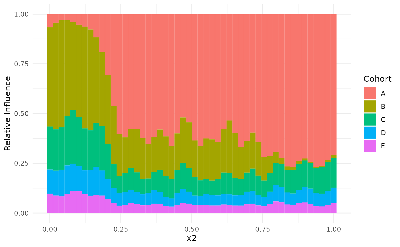
Create 5 datasets from standard gam example #1. The noise parameter is scaled, such that the first GAM has lowest noise and the last has highest noise. In a dominance plot, we plot the relative contributions of each dataset on the prediction. By the way we generated the data, we expect largest influence by dataset 1 and lowest by dataset 5.

## simulate datasets
set.seed(123)
datasets <- lapply(
  seq_len(num.datasets), 
  function(x) mgcv::gamSim(scale = x, verbose = FALSE))

Delete all data in the first dataset that has values lower than .2 on the dimension x2. Thus, we expect a low (i.e., zero) contribution of the first dataset on low values of dimensions x2.

df <- datasets[[1]]
df[df$x2<0.2,] <- NA
datasets[[1]] <- df

Next, delete all values of the second dataset for large values (x2>.8).

df <- datasets[[2]]
df[df$x2 > 0.8, ] <- NA
datasets[[2]] <- df

Fit GAMs

Next, we fit the individual GAMs for each of the eight datasets.

## fit a generalized additive model to each dataset separately
models <- lapply(datasets, function(dat){
  ## Full fit using mgcv
  gamfit <- mgcv::gam(y ~ s(x0, bs = "cr") + s(x1, bs = "cr") + s(x2, bs = "cr"), data = dat)
  ## Extract the necessary components for performing a meta-analysis
  ## This removes all subject-specific data
  strip_rawdata(gamfit)
})

If we also add names to the list of models, they will pop up as labels in dominance plots.

names(models) <- c("A", "B", "C", "D", "E")

Meta-Analysis

Then, we analyze the term s(x2). You can increase the resolution of the next plot by increasing grid_size, but we keep it low here to reduce the build time of the package.

meta_analysis <- metagam(models, grid_size = 50, terms = "s(x2)")

Dominance Analysis

Finally, we create a dominance plot that tells us how much the points on axis x2 are influenced by the individual GAMs. Since plot_dominance returns a ggplot object, we can modify the colors using, e.g. the viridis package. We see that the influence of the GAMs is graded according to the simulated noise levels. Second, we see that on the left-hand side, the influence of the first dataset is almost zero whereas the influence of the second dataset is almost zero on the righthand side.

plot_dominance(meta_analysis)